Manual
A theoretical background of Tikhonov regularization is provided in the The Inverse Problem section.
Solving a Problem
A problem consists of a design matrix ${\rm {\bf A}}$ and a vector ${\rm b}$ such that
\[{\rm b} = {\bf {\rm {\bf A}{\rm x}}} + \epsilon\]
where $\epsilon$ is noise and the objective is to reconstruct the original parameters ${\rm x}$. The solution to the problem is to minimize
\[{\rm {\rm x_{\lambda}}}=\arg\min\left\{ \left\lVert {\bf {\rm {\bf A}{\rm x}-{\rm b}}}\right\rVert _{2}^{2}+\lambda^{2}\left\lVert {\rm {\bf L}({\rm x}-{\rm x_{0}})}\right\rVert _{2}^{2}\right\} \]
where ${\rm x_{\lambda}}$ is the regularized estimate of ${\rm x}$, $\left\lVert \cdot\right\rVert _{2}$ is the Euclidean norm, ${\rm {\bf L}}$ is the Tikhonov filter matrix, $\lambda$ is the regularization parameter, and ${\rm x_{0}}$ is a vector of an a priori guess of the solution. The initial guess can be taken to be ${\rm x_{0}}=0$ if no a priori information is known.
The basic steps to solve the problem are
Ψ = setupRegularizationProblem(A, 2)   # Setup the problem
solution = solve(Ψ, b)                 # Compute the solution
xλ = solution.x                        # Extract the x
The solve function finds Optimal Regularization Parameter, by default using Generalized Cross Validation. It applies the optimal $\lambda$ value to compute ${\rm x}_\lambda$. The solution is of type RegularizatedSolution, which contains the optimal solution (solution.x), the optimal $\lambda$ (solution.λ) and output from the otimization routine (solution.solution).
An convenient way to find x is using Lazy pipes:
xλ = @> setupRegularizationProblem(A, 2) solve(b) getfield(:x)Specifying the Order
Common choices for the ${\bf{\rm{L}}}$ matrix are finite difference approximations of a derivative. There are termed zeroth, first, and second order inversion matrices.
\[{\rm {\bf L}_{0}=\left(\begin{array}{ccccc} 1 & & & & 0\\ & 1\\ & & \ddots\\ & & & 1\\ 0 & & & & 1 \end{array}\right)}\]
\[{\rm {\bf L}_{1}=\left(\begin{array}{cccccc} 1 & -1 & & & & 0\\ & 1 & -1\\ & & \ddots & \ddots\\ & & & 1 & -1\\ 0 & & & & 1 & -1 \end{array}\right)}\]
\[{\rm {\bf L}_{2}=\left(\begin{array}{ccccccc} -1 & 2 & -1 & & & & 0\\ & -1 & 2 & -1\\ & & \ddots & \ddots & \ddots\\ & & & -1 & 2 & -1\\ 0 & & & & -1 & 2 & -1 \end{array}\right)}\]
You can specify which of these matrices to use in
setupRegularizationProblem(A::AbstractMatrix, order::Int)where order = 0, 1, 2 corresponds to ${\bf{\rm{L}}_0}$, ${\bf{\rm{L}}_1}$, and ${\bf{\rm{L}}_2}$. Higher orders can be specified if desired.
Example : Phillips Problem
Example with 100 point discretization and zero initial guess.
using RegularizationTools, MatrixDepot, Lazy, DelimitedFiles
random(n) = @> readdlm("random.txt") vec x -> x[1:n]

r = mdopen("phillips", 100, false)
A, x = r.A, r.x

y = A * x
b = y + 0.1y .* random(100)
xλ = @> setupRegularizationProblem(A, 2) solve(b) getfield(:x)The example system is a test problem for regularization methods is taken from MatrixDepot.jl and is the same system used in Hansen (2000).
Example 2: Shaw Problem
Zeroth order example with 500 point discretization and moderate initial guess.
using RegularizationTools, MatrixDepot, Lazy, DelimitedFiles
random(n) = @> readdlm("random.txt") vec x -> x[1:n]

r = mdopen("shaw", 500, false)
A, x = r.A, r.x

y = A * x
b = y + 0.1y .* random(500)
x₀ = 0.6x

xλ = @> setupRegularizationProblem(A, 0) solve(b, x₀) getfield(:x)Using a Custom L Matrix
You can specify custom ${\rm {\bf L}}$ matrices when setting up problems.
setupRegularizationProblem(A::AbstractMatrix, L::AbstractMatrix)For example, Huckle and Sedlacek (2012) propose a two-step data based regularization
\[{\rm {\bf L}} = {\rm {\bf L}}_k {\rm {\bf D}}_{\hat{x}}^{-1} \]
where ${\rm {\bf L}}_k$ is one of the finite difference approximations of a derivative, ${\rm {\bf D}}_{\hat{x}}=diag(|\hat{x_{1}}|,\ldots|\hat{x_{n}}|)$, $\hat{x}$ is the reconstruction of $x$ using ${\rm {\bf L}}_k$, and $({\rm {\bf D}}_{\hat{x}})_{ii}=\epsilon\;\forall\;|\hat{x_{i}}|<\epsilon$, with $\epsilon << 1$.
Example 3: Heat Problem
This examples illustrates how to implement the Huckle and Sedlacek (2012) matrix. Note that Γ(n, 2) returns the Tikhonov Matrix of order 2.
using RegularizationTools, MatrixDepot, Lazy, LinearAlgebra, DelimitedFiles
random(n) = @> readdlm("random.txt") vec x -> x[1:n]

r = mdopen("heat", 100, false)
A, x = r.A, r.x

y = A * x
b = y + 0.04y .* random(100)
x₀ = zeros(length(b))

L₂ = Γ(length(b), 2)
xλ1 = @> setupRegularizationProblem(A, L₂) solve(b) getfield(:x)
x̂ = deepcopy(abs.(xλ1))
x̂[abs.(x̂) .< 0.1] .= 0.1
L = L₂*Diagonal(x̂)^(-1)
xλ2 = @> setupRegularizationProblem(A, L) solve(b) getfield(:x)The solution xλ2 is improved over the regular L₂ solution.
Adding Boundary Constraints
To add boundary constraints (e.g. enforce that all solutions are positive), the following procedure is implemented. Compute the algebraic solution without constraints, truncate the solution at the upper and lower bounds, and use the result as initial condition for solving the minimization problem with a least squares numerical solver LeastSquaresOptim. The regularization parameter λ obtained from the algebraic solution is used for a single pass optimization. See solve for a complete list of methods.
using RegularizationTools, MatrixDepot, Lazy, LinearAlgebra, DelimitedFiles
random(n) = @> readdlm("random.txt") vec x -> x[1:n]

r = mdopen("heat", 100, false)
A, x = r.A, r.x

y = A * x
b = y + 0.04y .* random(100)
x₀ = zeros(length(b))

L₂ = Γ(length(b),2)
xλ1 = @> setupRegularizationProblem(A, L₂) solve(b) getfield(:x)
x̂ = deepcopy(abs.(xλ1))
x̂[abs.(x̂) .< 0.1] .= 0.1
ψ = @>> L₂*Diagonal(x̂)^(-1) setupRegularizationProblem(A)
lower = zeros(100)
upper = ones(100)
xλ2 = @> solve(ψ, b, lower, upper) getfield(:x)This is the same example as above, but imposing a lower and upper bound on the solution. Note that this solve method computes the algebraic solution using solve(Ψ, b; kwargs...) method to compute the starting point for the least square minimization. You can also call
xλ2 = @> solve(ψ, b, x₀, lower, upper) getfield(:x)to bound the least-square solver by the output from the solve(Ψ, b, x₀; kwargs...) method.
Customizing the Search Algorithm
The solve function searches for the optimum regularization parameter $\lambda$ between $[\lambda_1, \lambda_2]$. The default search range is [0.001, 1000.0] and the interval range can be modified through keyword parameters. The optimality criterion is either the minimum of the Generalized Cross Validation function, or the the maximum curvature of the L-curve (see L-Curve Algorithm). The algorithm can be specified through the alg keyword. Valid algorithms are :L_curve, :gcv_svd, and :gcv_tr (see solve).
Example
using RegularizationTools, MatrixDepot, Lazy, DelimitedFiles
random(n) = @> readdlm("random.txt") vec x -> x[1:n]

r = mdopen("phillips", 100, false)
A, x = r.A, r.x

y = A * x
b = y + 0.1 .* random(100)

xλ1 = @> setupRegularizationProblem(A,1) solve(b, alg=:L_curve, λ₁=0.01, λ₂=10.0) getfield(:x)
xλ2 = @> setupRegularizationProblem(A,1) solve(b, alg=:gcv_svd, λ₁=0.01, λ₂=10.0) getfield(:x)Note that the output from the L-curve and GCV algorithm are nearly identical.
The L-curve algorithm is more sensitive to the bounds and slower than the gcv_svd algorithm. There may, however, be cases where the L-curve approach is preferable.
Extracting the Validation Function
The solution is obtained by first transforming the problem to standard form (see Transformation to Standard Form). The following example can be used to extract the GCV function.
using RegularizationTools, MatrixDepot, Lazy, Underscores, Printf, DelimitedFiles
random(n) = @> readdlm("random.txt") vec x -> x[1:n]

r = mdopen("shaw", 100, false)
A, x = r.A, r.x

y = A  * x
b = y + 0.05y .* random(100)

Ψ = setupRegularizationProblem(A,1)
λopt = @> solve(Ψ, b, alg=:gcv_svd) getfield(:λ)
b̄ = to_standard_form(Ψ, b)
λs = exp10.(range(log10(1e-1), stop = log10(10), length = 100))
Vλ = @_ map(gcv_svd(Ψ, b̄, _), λs)The calculated λopt from
λopt = @> solve(Ψ, b, alg=:gcv_svd) getfield(:λ)is 0.25 and corresponds to the minimum of the GCV curve.
Alternatively, the L-curve is retrieved through the L-curve Functions
using RegularizationTools, MatrixDepot, Lazy, Underscores, Printf, DelimitedFiles
random(n) = @> readdlm("random.txt") vec x -> x[1:n]

r = mdopen("shaw", 100, false)
A, x = r.A, r.x

y = A  * x
b = y + 0.05y .* random(100)

Ψ = setupRegularizationProblem(A,1)
λopt = @> solve(Ψ, b, alg=:L_curve, λ₂ = 10.0) getfield(:λ)
b̄ = to_standard_form(Ψ, b)
λs = exp10.(range(log10(1e-3), stop = log10(100), length = 200))
L1norm, L2norm, κ = Lcurve_functions(Ψ, b̄)
L1, L2 = L1norm.(λs), L2norm.(λs)The calculated λopt from
λopt = @> solve(Ψ, b, alg=:L_curve, λ₂ = 10.0) getfield(:λ)is 0.14 and corresponds to the corner of the L-curve.
The Invert Function
The code to perform second order regularization us
xλ = @> setupRegularizationProblem(A, 2) solve(b) getfield(:x)this can become a bit verbose, especially with more elaborate inversion methods. The invert function provides a high-level API. For example the code above can be written as
xλ = invert(A, b, Lₖ(2))here Lₖ(2) denotes the second order inversion and "2" is a hyperparameter that specifies the order. Several methods are predefined.
The method nomenclature is
Lₖfor regularization order (see Specifying the Order; the hyperparameter is the order k)Bfor bounded search (see Adding Boundary Constraints; the hyperparameters are the lower and upper bound, lb and ub)x₀for adding an intial guessDₓfor the Huckle and Sedlacek (2012) two-step data based regularization (see Using a Custom L Matrix; the hyperparameter is the noise level ε).
The InverseMethod data type takes the hyper parameters as arguments. The invert function passes all keyword arguments through to the solve function. Examples of method initializations are
# Hyper parameters
k: order, lb: low bound, ub: upper bound, ε: noise level, x₀: initial guess
k, lb, ub, ε, x₀ = 2, zeros(8), zeros(8) .+ 50.0, 0.02, 0.5*N

xλ = invert(A, b, Lₖ(k); alg = :gcv_tr, λ₁ = 0.1)
xλ = invert(A, b, Lₖ(k); alg = :gcv_svd, λ₁ = 0.1)
xλ = invert(A, b, LₖB(k, lb, ub); alg = :L_curve, λ₁ = 0.1)
xλ = invert(A, b, Lₖx₀(k, x₀); alg = :L_curve, λ₁ = 0.1)
xλ = invert(A, b, Lₖx₀(k, x₀); alg = :gcv_tr)
xλ = invert(A, b, Lₖx₀(k, x₀); alg = :gcv_svd)
xλ = invert(A, b, Lₖx₀B(k, x₀, lb, ub); alg = :gcv_svd)
xλ = invert(A, b, LₖDₓ(k, ε); alg = :gcv_svd)
xλ = invert(A, b, LₖDₓB(k, ε, lb, ub); alg = :gcv_svd)
xλ = invert(A, b, Lₖx₀Dₓ(k, x₀, ε); alg = :gcv_svd)
xλ = invert(A, b, Lₖx₀DₓB(k, x₀, ε, lb, ub); alg = :gcv_svd)
The formal definition of the InverseMethod data structure is
    @data InverseMethod begin
        Lₖ(Int)                              # Pure Tikhonov
        Lₖx₀(Int, Vector)                    # with initial guess
        LₖB(Int, Vector, Vector)             # with bounds
        Lₖx₀B(Int, Vector, Vector, Vector)   # with initial guess + bounds
        LₖDₓ(Int, Float64)                   # with filter
        Lₖx₀Dₓ(Int, Vector, Float64)         # with initial guess + filter
        LₖDₓB(Int, Float64, Vector, Vector)  # with filter + bound
        Lₖx₀DₓB(Int, Vector, Float64, Vector, Vector) # with initial guess + filter + bound
    end
Creating a Design Matrix
Standard Approach
This package provides an abstract generic interface to create a design matrix from a forward model of a linear process. To understand this functionality, first consider the standard approach to find the design matrix by discretization of the Fredholm integral equation.
Consider a one-dimensional Fredholm integral equation of the first kind on a finite interval:
\[\int_{a}^{b}K(q,s)f(s)ds=g(q)\;\;\;\;\;\;s\in[a,b]\;\mathrm{and}\;q\in[c,d]\]
where $K(q,s)$ is the kernel. The inverse problem is to find $f(s)$ for a given $K(q,s)$ and $g(q)$.
The integral equation can be cast as system of linear equations such that
\[\mathbf{A}\mathrm{x=b}\]
where $\mathrm{x}=[x_{1},\dots,x_{n}]=f(s_{i})$ is a discrete vector representing f, $\mathrm{b=}[b_{1},\dots,b_{n}]=g(q_{j})$ is a vector representing $g$ and $\mathrm{\mathbf{A}}$ is the $n\times n$ design matrix.
Using the quadrature method (Hansen, 2008), the integral is approximated by a weighted sum such that
\[\int_{a}^{b}K(q_{i},s)f(s)ds=g(q_{i})\approx\sum_{j=1}^{n}wK(q_{i},s_{j})f(s_{j})\]
where $w=\frac{b-a}{n}$, and $s_{j}=(j-\frac{1}{2})w$. The elements comprising the design matrix $\mathrm{\mathbf{A}}$ are $a_{i,j}=wK(q_{i},s_{j})$.
This simple kernel (Baart, 1982) serves as an illustrative example
\[K(q,s)=\exp(q\cos(s))\]
\[f(s)=\sin(s)\]
\[g(q)=\frac{2\sin s}{s}\]
\[s\in[0,\pi]\;\mathrm{and}\;q\in[0,\pi/2]\]
The following imperative code discretizes the problem with $n=12$ points:
a, b = 0.0, π
n, m = 12,12
c, d = 0.0, π/2
A = zeros(n,m)
w = (b-a)/n
baart(x,y) = exp(x*cos(y))
q = range(c, stop = d, length = n)
s = [(j-0.5)*(b-a)/n for j = 1:m]

for i = 1:n
    for j = 1:m
        A[i,j] = w*baart(q[i], (j-0.5)*w)
    end
end
In this example, the functions $f(s)$ and $g(q)$ are known. Evaluating $\mathrm{b}=\mathrm{\mathbf{A}x}$ with $\mathrm{\mathrm{x}}=sin(s)$ approximately yields $2sin(q)/q$.
x = sin.(s)
b1 = A*x
b2 = 2.0.*sinh.(q)./q
Here, b1 and b2 are close. However, as noted by Hansen (2008), the product $\mathbf{A}\mathrm{x}$ is, in general, different from $g(q)$ due to discretization errors.
Alternative Approach
Discretization of the kernel may be less straight forward for more complex kernels that describe physical processes. Furthermore, in physical processes or engineering systems, the mapping of variables isn't immediately clear. This is especially true when thinking about kernel functions of processes that have not yet been modeled in the literature.
Imagine the following problem studying a system of interest with some instrument. The instrument has a dial and intends to measure a physical property $x$ that is expressible as a numeric value. The dial can be any abstract notion such as "channel number", "input voltage", or even a combination of parameters such as "channel number 1 at high gain", "channel number 1 at low gain", and so forth. At each dial setting the instrument passes the physical property through a filter that produces an observable reading $b$. The domain of the problem consists of a list of valid set points $[s_{i}]$, with a corresponding list of physical properties $[x_{i}]$.
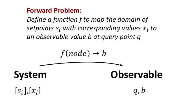
We can then defined a node element of the domain as a product data type
struct Domain{T1<:Any,T2<:Number,T3<:Any}
    s::AbstractVector{T1}
    x::AbstractVector{T2}
    q::T3
end
A single node in the domain is defined as
node = Domain([s], [x], q)where $q$ is an abstract query value of the instrument. The forward problem is to defined a function that maps a node of the domain to the observable $b$, i.e.
b = f(node) Here $b$ corresponds to a numerical value displayed by the detector at setting $q$.
The higher order function designmatrix
function designmatrix(s::Any, q::Any, f::Function)::AbstractMatrix
    n = length(s)
    x(i) = @_ map(_ == i ? 1.0 : 0.0, 1:n)
    nodes = [Domain(s, x(i), q[j]) for i ∈ 1:n, j ∈ 1:length(q)]
    return @> map(f, nodes) transpose copy
end
maps the list of setpoints s, query points q to the design matrix A for any function f(node) that can operate and the defined setpoints.
Then the $\mathrm{b}=\mathrm{\mathbf{A}x}$ is the linear transformation from a list of physical properties $[x_{i}]$ at query points $[q_{i}]$.
Below are three examples on how the function designmatrix works. Complete examples are included in the examples folder.
Example 1
Problem Setup
Consider a black and white camera taking a picture in a turbulent atmosphere. The camera has 200x200 pixel resolution. The input values to the camera correspond to the photon count hitting the detector. The output corresponds to a gray scale value between 0 and 1. Let us ignore other effects such as lens distortions, quantum efficiency of the detector, wavelength dependency, or electronic noise. However, the turbulent atmosphere will blur the image by randomly redirecting photons. The Gaussian blur kernel function is
\[K(x,y)=\frac{1}{2\pi\sigma}\exp\left(-\frac{x^{2}+y^{2}}{2\sigma^{2}}\right)\]
where x, y are the the distances from the pixel coordinate in the horizontal and vertical axis, and $\sigma$ is the standard deviation of the Gaussian distribution. The value of $K(x,y)$ is zero for pixels further than $x>c$ and $y>c$.
Each setpoint is $s_{i}$ is a tuple of physical coordinates (x,y). The domain for setpoints is a vector of tuples covering all pixels.
using Lazy

s = @> [(i,j) for i = 0:20, j = 0:20] reshape(:)
441-element Vector{Tuple{Int64, Int64}}:
(0, 0)
(1, 0)
(2, 0)
(3, 0)
(4, 0)
(5, 0)
(6, 0)
(7, 0)
(8, 0)
(9, 0)
⋮
(12, 20)
(13, 20)
(14, 20)
(15, 20)
(16, 20)
(17, 20)
(18, 20)
(19, 20)
(20, 20)The domain of query points $q_{i}$ are pixel coordinates. For this problem it is sensible that $[s]=[q]$, but this need not be the case. The function $f(node)\rightarrow b$ is obtained via
function get_domainfunction(σ, c)
    blur(x,y) = 1.0/(2.0*π*σ^2.0)*exp(-(x^2.0 + y^2.0)/(2.0*σ^2.0))

    function f(node::Domain)
        s, x, q = node.s, node.x, node.q
        x₁, y₁ = q[1], q[2]

        y = mapfoldl(+, 1:length(x)) do i
            x₀, y₀ = s[i][1], s[i][2]
            Δx, Δy = abs(x₁-x₀), abs(y₁-y₀)
            tmp = (Δx < c) && (Δy < c) ? blur(Δx,Δy) * x[i] : 0.0
        end
    end
end

f = get_domainfunction(2.0, 4)
Note that the function f is specialized for a particular σ and c value. The design matrix is then obtained via
s = @> [(i,j) for i = 0:20, j = 0:20] reshape(:)
q = s
A = designmatrix(s, q, f)
Finally, the blurred image is computed via
using Lazy

img = @> rand(21,21) reshape(:)
b1 = A*img
The design matrix is $n^2 \times n^2$, here 441 elements. The image is flattened to a 1D array and the blurred image is obtained via matrix multiplication.
Alternatively, this package provides the higher order function forwardmodel, which performs the equivalent calculation using the specialized function x.
function forwardmodel(
    s::AbstractVector{T1},
    x::AbstractVector{T2},
    q::AbstractVector{T3},
    f::Function,
)::AbstractArray where {T1<:Any,T2<:Number,T3<:Any}
    return @>> (@_ map(Domain(s, x, _), q)) map(f)
end
for example
b1 = A*img
b2 = forwardmodel(s, img, q, f)
and b1 and b2 are approximately equal.
Notes
The returned function $f$ is specialized for a specific value $\sigma$. In general, the forward model may depend on a substantial number of hyper parameters.
The setpoints $[s]$ and query points $[q]$ are interpreted by the function $f$. They therefore can by of any valid type.
The types if $[x]$ and $[b]$ need not be the same, although both must be a subtype of Number.
Unsurprisingly the matrix operation is much faster than the forwardmodel.
The matrix A can be used in principle to blur and deblur images. You can try it with tiny images. Unfortunately, even a small 200x200 pixel image produces a 40000x40000 matrix, which is too large for the algorithms implemented in this package.
The matrix A produced by the function designmatrix is by default a dense matrix. In practice the blur matrix of a well-ordered image is a Toeplitz matrix that can be stored in sparse format. The generic function cannot account for this.
The computation time using designmatrix is slower (or much slower for large images) than the explicit discretization of the kernel function.
Finally, the advantage of the designmatrix approach is to allow for easier conceptualization of the problem using type signatures and a declarative programming interface. This allows for factoring out some of the mathematical details of the discretization problem. It also immediately allows to apply the algorithm to non-square images nor does it rely on a particular sorting of the pixels to construct the matrix.
Example 2
Problem Setup
Consider a population of particles suspended in air. The particle size distribution is represented in 8 size channels between 100 and 1000 nm. The populations light scattering and light absorption properties are measured at 3 wavelength. The properties are the convolution between the particle size distribution and the optical properties determined by Mie theory.
\[\beta=\int_{D_{p1}}^{D_{p2}}Q\frac{dN}{dD_{p}}dD_{p}\]
where $Q$ is either the scattering or absorption cross section of the particle that can be computed from Mie theory, represented through a function Mie(ref,Dp,λ), which is a function of the complex refractive index of the particle ($ref$), particle diameter ($D_{p}$), and wavelength ($\lambda$). Integration is performed over the size distribution $\frac{dN}{dD_{p}}$ and the interval $[D_{p1},D_{p2}]$. In this example, the domain $[s]$ comprises the 8 particle diameters
include("size_functions.jl") # hide

s = zip(["Dp$i" for i = 1:length(Dp)],Dp) |> collect
8-element Vector{Tuple{String, Float64}}:
("Dp1", 115.4781984689458)
("Dp2", 153.9926526059492)
("Dp3", 205.3525026457146)
("Dp4", 273.8419634264361)
("Dp5", 365.1741272548377)
("Dp6", 486.9675251658631)
("Dp7", 649.3816315762112)
("Dp8", 865.9643233600654)The setpoints $[s]$ are an array of tuples with labeled diameter and midpoint diameters in units of [nm].
The query points are the scattering and absorption cross sections measured at three different wavelength
q = [q1; q2]6-element Vector{Tuple{String, Float64}}:
("βs300", 3.0e-7)
("βs500", 5.0e-7)
("βs900", 9.0e-7)
("βa300", 3.0e-7)
("βa500", 5.0e-7)
("βa900", 9.0e-7)Thus the query points $[q]$ are an array of tuples with labels and wavelengths in units of [m]. Note that $\beta_s$ denotes scattering and $\beta_a$ the absorption cross section of the aerosol.
The design matrix is obtained via
function get_domainfunction(ref)
    function f(node::Domain)
        s, x, q = node.s, node.x, node.q
        Dp, λ = (@_ map(_[2], s)), q[2]

        Q = @match q[1][1:3] begin
            "βs" => @_ map(Qsca(π*Dp[_]*1e-9/λ, ref), 1:length(Dp))
            "βa" => @_ map(Qabs(π*Dp[_]*1e-9/λ, ref), 1:length(Dp))
            _ => trow("error")
        end
        mapreduce(+, 1:length(Dp)) do i
            π/4.0 *(x[i]*1e6)*Q[i]*(Dp[i]*1e-6)^2.0*1e6
        end
    end
end

f = get_domainfunction(complex(1.6, 0.01))
note that Qsca and Qabs are functions that return the scattering and absorption cross section from Mie theory for a given size parameter and refractive index. The domain function f is specialized for the refractive index n = 1.6 + 0.01i".
The matrix is obtained via
Dp, N = lognormal([[100.0, 500.0, 1.4]], d1 = 100.0, d2 = 1000.0, bins = 8)

A = designmatrix(s, q, g)
b = A*N
The matrix A is 6x8. N are the number concentrations of at each size (length 8). A*N produces 6 measurements corresponding to three $\beta_s$ and three $\beta_a$ values.
In this example 8 sizes are mapped to 6 observations. The setpoint $[s]$ and query $[q]$ domains are distinctly different in type.
The input and output tuples annotate data. The annotations are interpreted by the domain function to decide which value to compute (scattering or absorption).
This "toy" example illustrates the advantage of the domainmatrix discretization method. Only a few lines of declarative code are needed to compute converted to the domain matrix, even though the underlying model is reasonably complex. There is need to explicitly write out the equations to discretize the domain.
Example 3
This example is the implementation of the Baart (1982) kernel shown in the beginning.
\[K(q,s)=\exp(q\cos(s))\]
In this example, the domain $[s]$ comprises the integration from $[0..\pi]$
s = range(0, stop = π, length = 120)
q = range(0, stop = π/2, length = 120)
The forward model domain function is
function get_domainfunction(K)
    function f(node::Domain)
        s, x, q = node.s, node.x, node.q
        Δt = (maximum(s) - minimum(s))./length(x)
        y = @_ mapfoldl(K(q, (_-0.5)*Δt) * x[_] * Δt, +, 1:length(x))
    end
end
The design matrix is obtained via
f = get_domainfunction((x,y) -> exp(x*cos(y)))
A = designmatrix(s, q, f)
Again, in this the solution is knonw. Evaluating $\mathrm{b}=\mathrm{\mathbf{A}x}$ with $\mathrm{\mathrm{x}}=sin(s)$ approximately yields $2sin(q)/q$.
x = sin.(s)
b1 = A*x
b2 = 2.0.*sinh.(q)./q
And again b1 and b2 are close. Also A computed using the designmatrix function is the same than the explicit integration by quadrature.
Benchmarks
Systems up to a 1000 equations are unproblematic. The setup for much larger system slows down due to the $\approx O(n^2)$ (or worse) time complexity of the SVD and generalized SVD factorization of the design matrix. Larger systems require switching to SVD free algorithms, which are currently not supported by this package.
using RegularizationTools, TimerOutputs, MatrixDepot, Memoize

to = TimerOutput()

function benchmark(n)
    r = mdopen("shaw", n, false)
    A, x = r.A, r.x
    y = A * x
    b = y + 0.05y .* randn(n)
    Ψ = setupRegularizationProblem(A, 2)
	empty!(memoize_cache(setupRegularizationProblem))
    for i = 1:1
        @timeit to "Setup  (n = $n)" setupRegularizationProblem(A, 2)
        @timeit to "Invert (n = $n)" solve(Ψ, b)
    end
end

benchmark(10)
benchmark(100)
benchmark(1000)
show(to)
[ Info: Precompiling TimerOutputs [a759f4b9-e2f1-59dc-863e-4aeb61b1ea8f]
────────────────────────────────────────────────────────────────────────────
Time Allocations
────────────────────── ───────────────────────
Tot / % measured: 7.29s / 36.2% 839MiB / 35.2%
Section ncalls time %tot avg alloc %tot avg
────────────────────────────────────────────────────────────────────────────
Setup (n = 1000) 1 2.51s 95.2% 2.51s 269MiB 91.0% 269MiB
Invert (n = 1000) 1 90.5ms 3.42% 90.5ms 23.0MiB 7.77% 23.0MiB
Setup (n = 100) 1 25.1ms 0.95% 25.1ms 2.82MiB 0.95% 2.82MiB
Setup (n = 10) 1 7.70ms 0.29% 7.70ms 51.1KiB 0.02% 51.1KiB
Invert (n = 100) 1 3.88ms 0.15% 3.88ms 779KiB 0.26% 779KiB
Invert (n = 10) 1 172μs 0.01% 172μs 57.8KiB 0.02% 57.8KiB
────────────────────────────────────────────────────────────────────────────